This was my first ever machine learning project for my introduction to statistical machine learning class at UCSB. CS:GO was a favorite game of mine for years and while I hate the idea of gambling, it felt like an exciting opportunity to explore an area where I could develop something that might be able to produce positive EV. The heavy lifting and portion of this project that I’m actually proud of is the feature engineering. While it was certainly the most confusing and frustrating part (self-induced by being unorganized with my preprocessing), it was also the element that made me realize the creativity involved in data science for feature selection. On the modeling side of this, I definitely didn’t leave myself enough time and didn’t realize until far too late that somewhere in my preprocessing stage, I had leaked my response into my data resulting in horribly overfit models. I spent 36 hours desperately trying to identify where the response was leaked, but to no avail. This taught me how essential having an organized pre-processing stage for my data is (although it took another traumatic experience with my future chess projects to have the lesson really settle). Finally, reading back over this made me realize how horrifically I had presented this. If I were to redo this, there’s a lot I would do differently, but the presentation especially would need to be a 10000 times more readable and more organized.

Introduction

Counter-Strike (or CSGO/CS2 as it is commonly referred to as) is a popular first-person shooter which with its rise in popularity has had a pro scene grow in parallel to it. A classic problem within any professional scene (or really any event which is uncertain and has a large following) is being able to predict the outcome of the event usually for the purpose of betting. Additionally, the use of data science within professional sports has been growing so fora team to gain insights into what caused them to lose is of extreme importance.

Most matches in CSGO have multiple rounds which teams play. We will not be trying to predict overall match outcomes for this project, but rather individual match outcomes. While predicting the outcome of a match might seem like a highly daunting task, I tried to simplify it slightly in order to make it easier to think about the problem. There seemed to be three principle components as such:

Match Outcome = Relative Form + Map-Specific Features + Historical Matchup

Let’s break down exactly what I mean with each of these terms:
Relative Form: This is a measure of the difference in recent performance between the two teams. This ideally should be a measure of the trailing average across multiple relevant metrics that displays whether the form has been performing well or poorly.
Map-Specific Features: There are many different maps in CSGO and a team might be better on a certain map compared to others. Therefore there may be factors related to the match outcome that are map-specific.
Historical Matchup: When two teams face off, it might be the case that there are certain factors related to the two teams inconsideration and how they’ve historically performed against each other that exist independent of overall form and the map which need to be considered.

First we will load in our necessary packages and our dataset. The dataset we sourced was from aggregated from hltv.org by Mateus Dauernheimer Machado as a dataset available to be used on Kaggle.

Mateus’s Kaggle Post: https://www.kaggle.com/datasets/mateusdmachado/csgo-professional-matches

From Mateus’s dataset, we completely transformed the data in order to create more useful predictors for match outcomes. When predicting the outcomes of these games, the only data that we have to work off of is historical data, and as such, it was necessary to construct custom trailing predictors for each match. Constructing this new dataset took a majority of the work for this project.

Missing Data:

During the reconstruction of Mateus’s dataset, unfortunately many games were lost from consideration in the model during the process of building our new dataset. Games from 2015 to the beginning of 2017 were lost due to the fact that HLTV did not collect economic data from the matches, a critical component we consider in our analysis of the games. Because imputation for a set of over 20000 games would be absolutely ridiculous, it made more sense to cut them out, leaving me with around 29000 matches. Now, when I rebuilt the dataset, it cannot be understated how complicated this process was. While I paid careful attention to how I needed to join our tables in order to get the dataset in a format that would be useful to me, there were obvious mistakes I made in the process and due to a lack of experience and time, concessions had to be made. In order to make sure that all the data that I had careful crafted over months maintained the properties seen in the original dataset, I had to end up deleting close to 24000 matches. This leaves us with roughly 6000 matches, but that’s enough!

In the resulting dataset, there is no missing data. All NA values were omitted due to the fact that I didn’t feel comfortable imputing results in when the dynamics for each team are so radically different. With that said, we don’t need to worry about missing data in our project. When checking the win rate distribution across teams, we observed that team 1 won 54% of the time, indicating a considerable imbalance. When checking the original data, this result is also present however is not as pronounced. To fi x this issue, we will oversample matches where team 2 wins when constructing our training and testing sets. Before we do that though, let us first investigate the data and make inferences about what our model should look like.

EDA:

Now it’s time to get to work on figuring out what determines the winner of a CSGO match… on average. In order to first get a bird’s eye view over our predictors, let’s look at a correlation matrix with all our predictors:

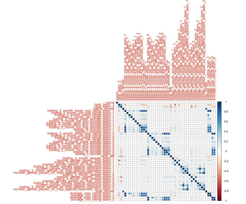
When looking at the correlation plot with specifi cally our two variables of interest, map_winner and match_winner,something which was quite interesting to observe was the lack of correlation between the map and opponentspecifi c features for each team and their winning. Initially when planning this project, I believed that these wouldbe our strongest predictors, however it might make sense that the factors related to these would be the fi rst thateach team would investigate when preparing for the match, so they would end up not playing much of a role indeciding the winner.

Without a doubt, the most surprising element that I noticed here was that the trailing average win rate on the map, in general, against the other team, and on the map against the opponent seemed to have among the least correlation with match winner for all. This made me suspicious that something might be wrong with my data, but I would have to wait until later to confirm.

We notice that the predictor with the largest absolute correlation (aside from map_winner which we will not be using) is the rank difference between teams, and that makes sense! With the way that the predictor is built (team1 rank – team 2 rank, noting that lower rank is actually better), a positive value implies that team 1 is actually the underdog while a negative value implies that team 2 is the underdog. A higher value of match_winner means that team 2 won, and it would seem logical that if team 1 is the underdog, team 2 would be more likely to win and vice versa for when team 1 wins and team 2 is the underdog. Let’s then dig a little deeper into rank difference in relation to our other factors. How about general team breakdowns? How does the average winning team compare to the losing team? Are there any noticeable inferences we can make?

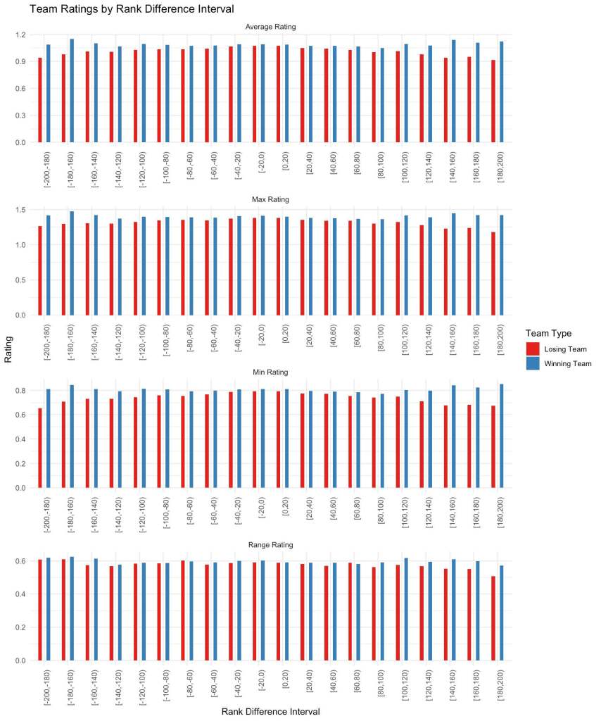
Okay, so while might seem confusing, let’s break it down because it’s actually quite useful to see. Remember that rank_diff is calculated as rank_team_1 – rank_team_2 and because a lower rank is better, positive values are where team 1 is the underdog and negative values are where team 2 is the underdog. With that in mind, we notice that when the difference in rank between teams is small, there’s general a smaller difference average team rating, min player rating, max player rating, and the range in team performance. When the rank difference becomes large, we see that there becomes a large difference between the two teams’ performance metrics. We will use this result to generate a useful interaction variable.

Now we notice a few irregularities such as for the range, it seems as though there’s a dip in the average range for the losing team when team 1 is the underdog while we don’t have a similar pattern when team 2 is the underdog. Unfortunately there’s nothing we can really do to investigate this further, however in our model results we will check if this had a material influence on our results.

Let’s examine our primary metrics of performance with relation to rank difference given that a team won or lost. In Counter Strike, teams receive virtual money for accomplishing certain goals among other factors. Depending on how much money you have, you can purchase different equipment to play with each round. Based on the aggregate equipment value, we classify these rounds as either a pistol, full-eco, semi-eco, semi-buy, or full-buy round. Because professional teams have proper economy management (and by design of the game), the vast majority of rounds are full-buy rounds and these are the most important to consider.

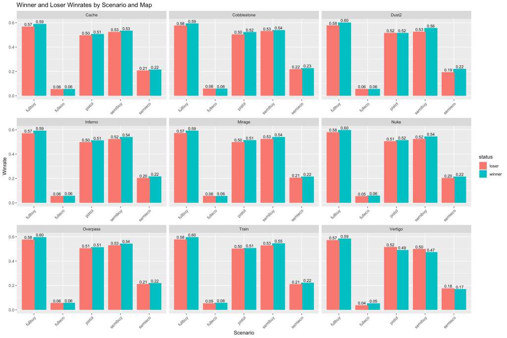
Interesting! So it appears that regardless of the map we’re looking at, the significance of each type of economy-round classification is fairly similar. As expected, full-buy rounds are the most important along with pistol and semi-buy while semi-eco and full-eco are far below. More importantly though, there seems to be a very small difference between all of the metrics for the winners and losers on all of the maps. This indicates to us that having interactions between these variables is not necessary.

Another element of the game which adds more to the depth of the game is the fact that there are two different sides to play on: terrorist and counter-terrorist. Terrorists aim to plant a bomb on a site while counter-terrorists try to prevent that. This is a crucial element to gameplay as it affects who is attacking versus who is defending, and the economic and play-style considerations as a result change dramatically. Let’s see how this is affected, first by different map:

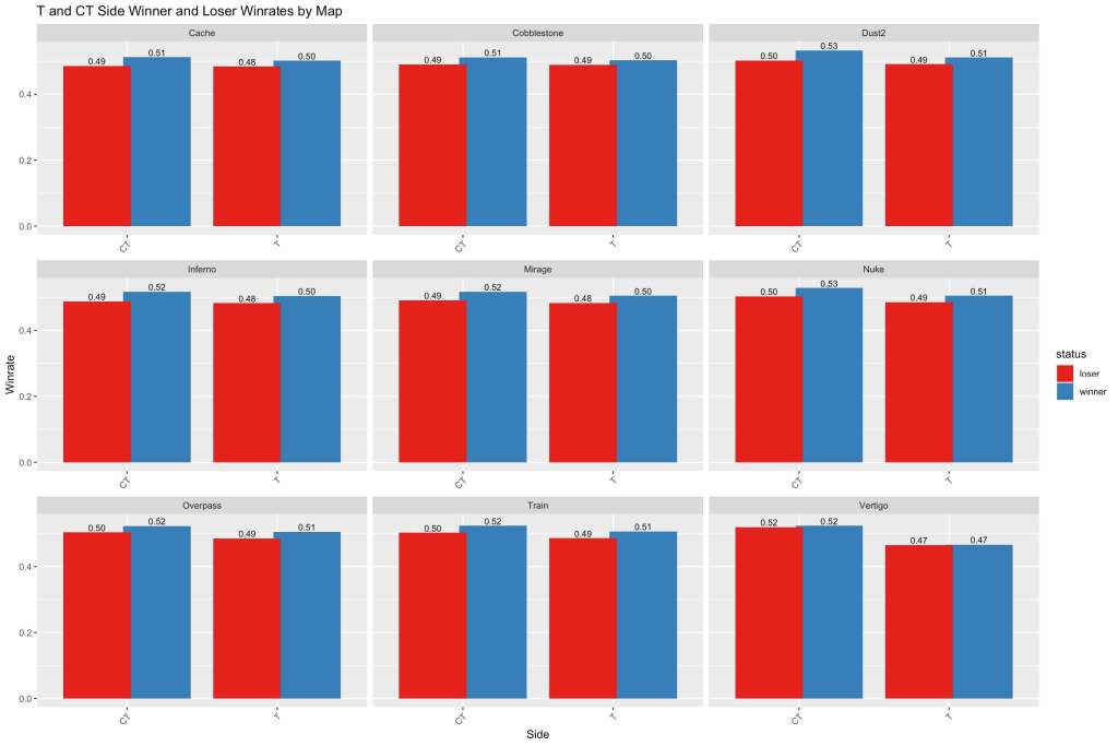
Again, we see limited difference between the teams, however there still does exist a persistent difference! For one, it appears that in general it is more important for a team to be stronger on the CT side as opposed to the T side. The insight that this gives us though in terms of our recipe is that we will not be including an interaction between.

The rest of our factors don’t seem to hold as much significance so we’ll be moving on, however clearly there’s still a lot of very interesting insights to be uncovered!

Modeling:

First we create our samplings. We will be using stratified sampling with our training and testing sets to ensure that we have comparable representation of match winner between the 2 teams.

Now we create our recipe for the models. When creating our recipe, we will be using the insights we gained from our EDA to generate a model that is built around our findings. The primary inclusion to our model that we will do is to include interactions between our performance variables and the rank difference. Our model is as follows:

Recipe creation and prep

model_recipe = recipe(match_winner~.,data=training) %>%
step_interact(terms = ~ rank_diff:trailing_3_month_mean_avg_rating_team_1) %>%
step_interact(terms = ~ rank_diff:trailing_3_month_mean_avg_rating_team_2) %>%
step_interact(terms = ~ rank_diff:average_min_rating_team_1) %>%
step_interact(terms = ~ rank_diff:average_min_rating_team_2) %>%
step_interact(terms = ~ rank_diff:average_max_rating_team_1) %>%
step_interact(terms = ~ rank_diff:average_max_rating_team_2) %>%
step_interact(terms = ~ rank_diff:trailing_3_month_mean_range_team_1) %>%
step_interact(terms = ~ rank_diff:trailing_3_month_mean_range_team_2)

For this project, four models were implemented:

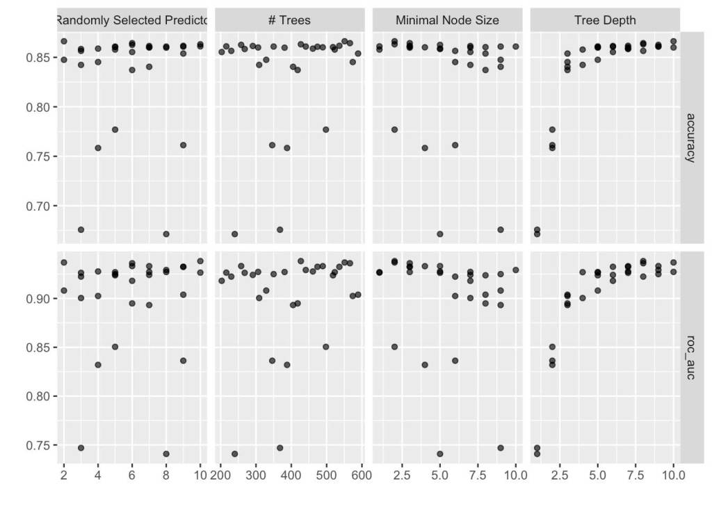
Random Forest: A powerful ensemble model which is able to generate trees by analyzing relationships between the predictors selected. It produces trees independently and for our purpose will be used to classify whether team1 or team 2 will win the match.

K Nearest Neighbors: A method for classification and regression which utilizes a clustering technique to predict the class a point belongs to. The parameter being tuned in this case is the number of neighbors, which is the number of nearby points to group together to make a prediction.

Gradient Boosted Trees: Another ensemble method similar to the Random Forest method, however uses boosted trees which can be more susceptible to over-fitting. With our gradient boosted trees, we will be tuning 2 of our hyperparameters: min_n and trees. Trees is just the number of trees that we see in our model while min_n is the minimum number of nodes present for a tree to continue splitting down. This was the most intensive model to generate, so I utilized parallel processing to make it run faster (not important to this class but was cool to learn about and implement on my own).

Logistic Regression: A method used for regression as well as classification (contrary to what its name might suggest). We tune the penalty parameter with our regression in order to reduce the amount of complexity with the model and hopefully obtain something more realistic.

Now let’s check the results we obtained from each one of our models. First we will load in the results that we obtained and saved.

Random Forest:

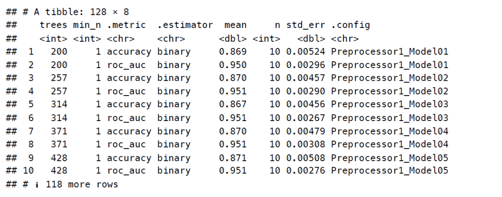
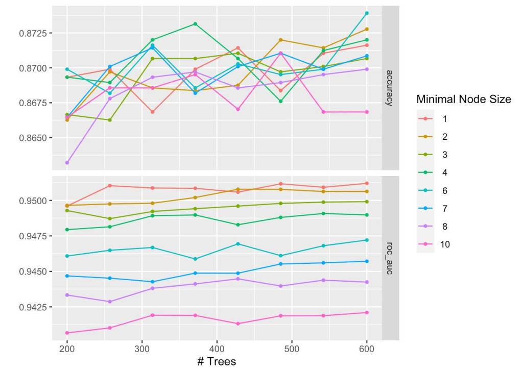
An interesting result we seem to get is that all of our models on our trained set have very high accuracy, however based on the number of trees we have, as we increase the minimal node size, we see a strict (albeit slight)reduction in ROC AUC scores. We will end up choosing our RF model with a minimal node size of 1 and with 600 trees. With our cross validation, we end up seeing that our mean ROC AUC scores were around 90% with an average standard error of around 0.004, indicating that the models learned very well how to predict the data.

K Nearest Neighbors:

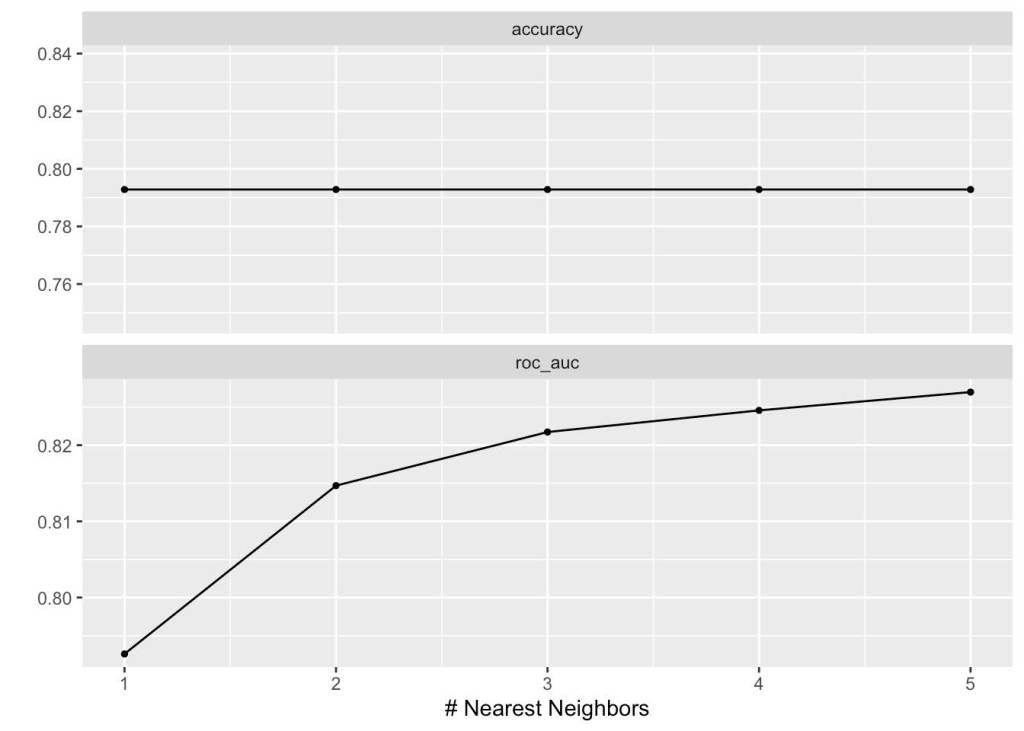
For our KNN, we see that as the number of neighbors increases, we improve the ROC AUC score by a maximum of 5% to 83.4%, however our accuracy remains basically constant. This doesn’t seem as likely to be overfit based on the score observed. This result, while not as fantastic as our random forest model, seems much more realistic.

Gradient Boosted Trees:

Looking at our results, it’s extremely likely the model overfit to the data. Our ROC AUC and accuracy both increased as we increased tree depth to over 90%. Considering a feature of gradient boosted trees it that they improve on previous iterations of themselves, it also explains why we see almost a ratcheting up of accuracy and ROC AUC as we increase the depth. While the results are obviously stellar, we can’t really rely on them as they seem to be too closely fit.

Logistic Regression

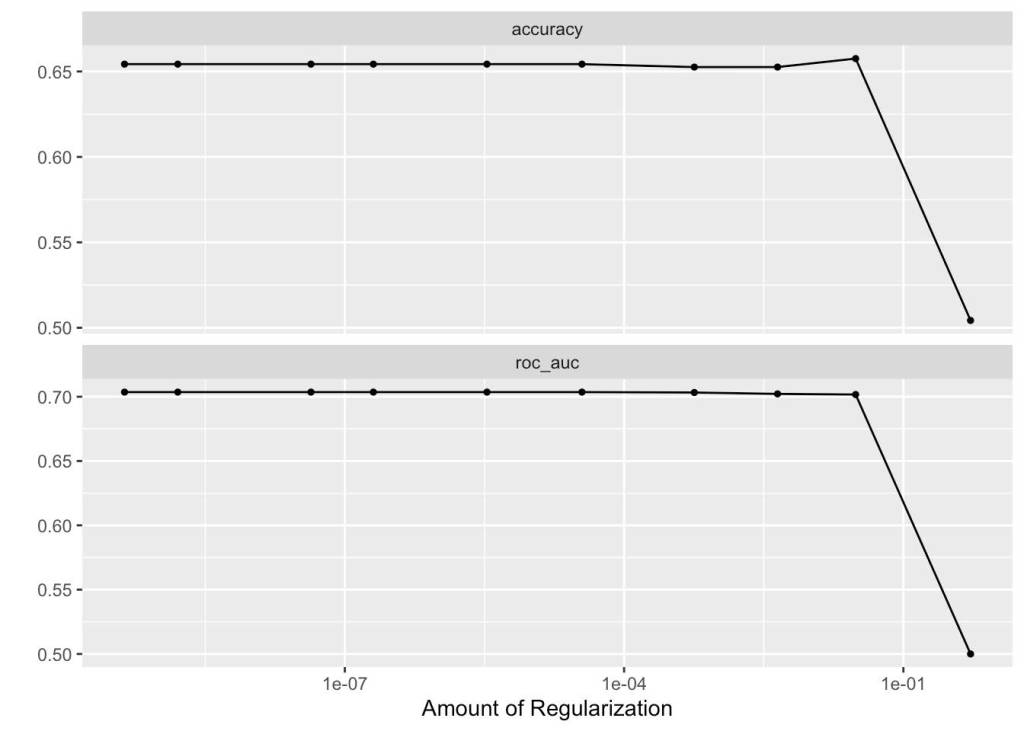
Our logistic regression has a considerably lower accuracy attached to it. We notice that while the accuracy and ROC AUC for the most part stay stagnant around 65% and 71% respectively, as soon as our regularization hits a certain threshold they both drop off considerably. This is because the regularization penalty drives down the influence of our individual predictors as it increases in hopes of generating a more simple model. It tells us that our predictors might not have as much influence as they seem to, up until a certain point where the over-penalization becomes detrimental.

Testing

Our best result by far was the random forest and gradient-boosted trees. Both of these unfortunately were clearly overfit, however I did not have enough time to properly address what the issue ended up being. In order to prevent this, multiple methods could be implemented such as increasing the number of trees.

We will apply 2 of our models to our testing set. One will be the random forest model and the other will be our logistic regression model. The reason I chose these 2 was because while my random forest model appeared the best, it also appeared overfit. The logistic regression did not have as much overfitting present, and thus I want to see how it compares to the testing set.

Logistic Regression

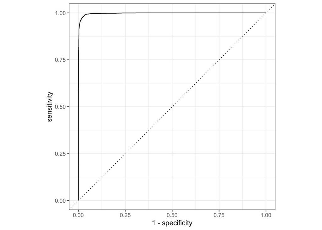
Random Forest

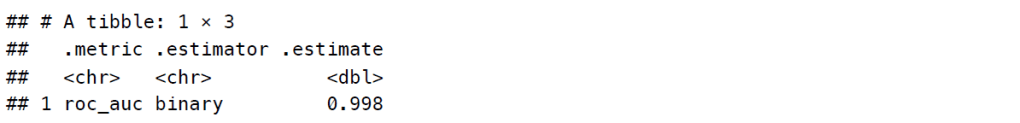
Our plots look promising, although again way too accurate. Let’s see our overall scores:

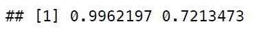
Our final result is a little frustrating. Whether we choose to use our random forest model whose results are scarily accurate, suggesting an error in our data, or whether we choose our logistic regression model whose results are more realistic although still very similar to the testing data, the outcomes are not too different from our training data. It might be the case that as a result of the data we picked in our project, the games that survived our data preprocessing stage have a large amount of correlation that aren’t apparent. Regardless, this was a very fun project and one which taught me principles of machine learning which I plan on using in the future as well as more about a game I thought already knew everything about!